#read in West coast EEZ shape file w terra
wc_EEZ_regions <- st_read(here("posts",
"2022-12-03_geospatial",
"data",
"wc_regions_clean.shp"))
#read in SST rasters
avg_sst_2008 <- rast(here("posts",
"2022-12-03_geospatial",
"data",
"average_annual_sst_2008.tif"))
avg_sst_2009 <- rast(here("posts",
"2022-12-03_geospatial",
"data",
"average_annual_sst_2009.tif"))
avg_sst_2010 <- rast(here("posts",
"2022-12-03_geospatial",
"data",
"average_annual_sst_2010.tif"))
avg_sst_2011 <- rast(here("posts",
"2022-12-03_geospatial",
"data",
"average_annual_sst_2011.tif"))
avg_sst_2012 <- rast(here("posts",
"2022-12-03_geospatial",
"data",
"average_annual_sst_2012.tif"))
#combine into raster stack
all_sst <- c(avg_sst_2008,
avg_sst_2009,
avg_sst_2010,
avg_sst_2011,
avg_sst_2012)
#read in bathymetry raster
depth <- rast(here("posts",
"2022-12-03_geospatial",
"data",
"depth.tif"))Background
This blog post is from my Geospatial Analysis and Remote Sensing course as a part of my master’s program at the Bren School for Environmental Science & Management. I will be determining which Exclusive Economic Zones (EEZ’s) on the West Coast of the United States are the most suitable for developing marine aquaculture for many species of oysters. Then, I make a function to map any species’ suitable habitats within West Coast EEZs by allowing for user inputs of species’ suitable habitats based on sea surface temperatures and depth.
Data
Sea Surface Temperature Data
I will use average annual sea surface temperature (SST) from the years 2008 to 2012 to characterize the average sea surface temperature within the region. The data we are working with was originally generated from NOAA’s 5km Daily Global Satellite Sea Surface Temperature Anomaly v3.1.
Bathymetry Data
To characterize the depth of the ocean, I will use the General Bathymetric Chart of the Oceans (GEBCO).[^3]
Exclusive Economic Zones Data
We will be designating maritime boundaries using Exclusive Economic Zones off of the west coast of US from Marineregions.org.
Process
I will start with loading the necessary data listed above and validate that all the data has the same coordinate reference system.
Checking if the coordinate reference systems are the same. The sea surface temperature data needs to be reprojected to match the coordinate reference systems of the EEZ and depth data.
st_crs(wc_EEZ_regions) # crs EPSG:4326Coordinate Reference System:
User input: WGS 84
wkt:
GEOGCRS["WGS 84",
DATUM["World Geodetic System 1984",
ELLIPSOID["WGS 84",6378137,298.257223563,
LENGTHUNIT["metre",1]]],
PRIMEM["Greenwich",0,
ANGLEUNIT["degree",0.0174532925199433]],
CS[ellipsoidal,2],
AXIS["latitude",north,
ORDER[1],
ANGLEUNIT["degree",0.0174532925199433]],
AXIS["longitude",east,
ORDER[2],
ANGLEUNIT["degree",0.0174532925199433]],
ID["EPSG",4326]]st_crs(all_sst) #crs EPSG:9122Coordinate Reference System:
User input: WGS 84
wkt:
GEOGCRS["WGS 84",
DATUM["unknown",
ELLIPSOID["WGS84",6378137,298.257223563,
LENGTHUNIT["metre",1,
ID["EPSG",9001]]]],
PRIMEM["Greenwich",0,
ANGLEUNIT["degree",0.0174532925199433,
ID["EPSG",9122]]],
CS[ellipsoidal,2],
AXIS["latitude",north,
ORDER[1],
ANGLEUNIT["degree",0.0174532925199433,
ID["EPSG",9122]]],
AXIS["longitude",east,
ORDER[2],
ANGLEUNIT["degree",0.0174532925199433,
ID["EPSG",9122]]]]st_crs(depth) #crs EPSG 4326Coordinate Reference System:
User input: WGS 84
wkt:
GEOGCRS["WGS 84",
ENSEMBLE["World Geodetic System 1984 ensemble",
MEMBER["World Geodetic System 1984 (Transit)"],
MEMBER["World Geodetic System 1984 (G730)"],
MEMBER["World Geodetic System 1984 (G873)"],
MEMBER["World Geodetic System 1984 (G1150)"],
MEMBER["World Geodetic System 1984 (G1674)"],
MEMBER["World Geodetic System 1984 (G1762)"],
MEMBER["World Geodetic System 1984 (G2139)"],
ELLIPSOID["WGS 84",6378137,298.257223563,
LENGTHUNIT["metre",1]],
ENSEMBLEACCURACY[2.0]],
PRIMEM["Greenwich",0,
ANGLEUNIT["degree",0.0174532925199433]],
CS[ellipsoidal,2],
AXIS["geodetic latitude (Lat)",north,
ORDER[1],
ANGLEUNIT["degree",0.0174532925199433]],
AXIS["geodetic longitude (Lon)",east,
ORDER[2],
ANGLEUNIT["degree",0.0174532925199433]],
USAGE[
SCOPE["Horizontal component of 3D system."],
AREA["World."],
BBOX[-90,-180,90,180]],
ID["EPSG",4326]]#re project using the terra way
all_sst_reproj <- project(all_sst,
wc_EEZ_regions)Process data
Next, I need process the SST and depth data so that they can be combined, I will resample to match the SST data using the nearest neighbor approach since the extents, resolutions, and positions of the depth and SST are different.
#find the mean SST from 2008-2012
mean_sst <- mean(all_sst_reproj)
#convert sst from K to C
mean_sst_c <- mean_sst - 273.15#crop depth rast to match the extent of the SST rast
depth_cropped <- crop(depth,mean_sst_c)
#using nearest neighbor approach to resample
depth_resampled <- resample(depth_cropped,
mean_sst_c,
method = "near")
#stack to check if they have the same resolution
resolution_test <- c(depth_resampled,
all_sst_reproj)
#they stacked properly, indicating that they both have same resolutions, extent, and crsFind suitable locations
To determine suitable locations for marine aquaculture, I need to look for locations that are suitable in terms of both SST and depth.
#oyster happy spots
#sea surface temperature: 11-30°C\
#depth: 0-70 meters below sea level
#reclassify sst into suitable locations for oysters
#reclassification matrix for suitable range of sst
rcl_sst <- matrix(c(-Inf, 11, NA, 11, 30,
1,30, Inf, NA),
ncol = 3, byrow = TRUE) #anything outside of range is NA
#reclassifying raster using a reclassification matrix
sst_suitable_locs <- classify(mean_sst_c,
rcl = rcl_sst,
include.lowest = TRUE)#reclassify depth into suitable locations for oysters
#reclassification matrix for suitable range of depths
rcl_depth <- matrix(c(-Inf, -70, NA,
-70, 0, 1,
0, Inf, NA),
ncol = 3, byrow = TRUE)
#reclassifying raster using a reclassification matrix
depth_suitable_locs <- classify(depth_resampled,
rcl = rcl_depth,
include.lowest = TRUE)#define function
mult_fun <- function(x, y) {
return(x*y)}
#find locations that satisfy both conditions
oyst_suitable_habitat <- lapp(c(sst_suitable_locs, depth_suitable_locs), mult_fun)Determining the most suitable EEZ
I want to determine the total suitable area within each EEZ so I can rank zones by priority. To do this, I will need to find the total area of suitable locations within each EEZ.
# making obj of individual cell size of areas that are suitable for oysters so we can find the size of each cell
grid_cell_size <- cellSize(oyst_suitable_habitat,
mask = TRUE, #keep values within the suitable habitat
transform = TRUE,
unit = "km")
plot(grid_cell_size, main = "Cell Size")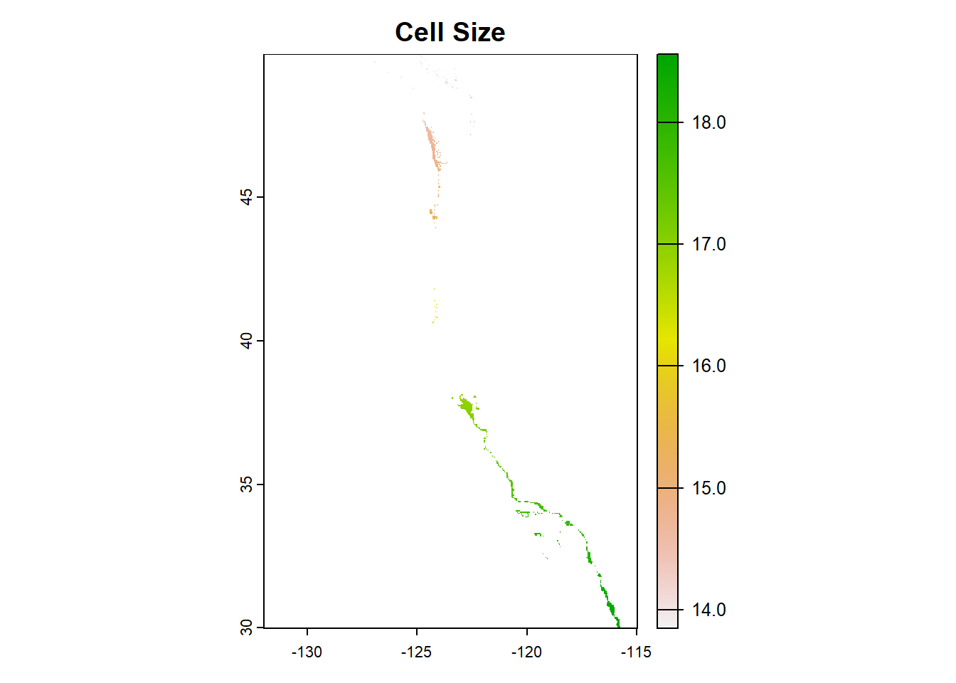
# rasterize wc shape file to help find total suitable area
# Rasterize(): Transfer values associated with 'object' type spatial data (points, lines, polygons) to raster cells.
# wc_EEZ regions are the points, and we will transfer those values to the raster i set up earlier for suitable oyster habitats
wc_rasterized <- rasterize(wc_EEZ_regions,
oyst_suitable_habitat,
field = "rgn")#make a mask of wc raster and suitable locs for oysters
#goal is to have areas of suitable oyster habitat that also fall in w coast EEZ regions
wc_mask <- mask(wc_rasterized, oyst_suitable_habitat,
updatevalue = NA,
inverse = FALSE)#find area of each suitable zones with zonal() in each of 5 regions of EEZ
wc_suitable_area <- zonal(grid_cell_size, wc_mask, na.rm = TRUE, sum)#join data
wc_suitable_EEZ <- full_join(wc_EEZ_regions, wc_suitable_area, by = "rgn") |>
mutate(suitable_area = area, #rename area to suitable area
percentage_suitable = (suitable_area/area_km2 * 100), #percentage of suitable area
.before = geometry)
print(wc_suitable_EEZ)Simple feature collection with 5 features and 8 fields
Geometry type: MULTIPOLYGON
Dimension: XY
Bounding box: xmin: -129.1635 ymin: 30.542 xmax: -117.097 ymax: 49.00031
Geodetic CRS: WGS 84
rgn rgn_key area_m2 rgn_id area_km2 area
1 Oregon OR 179994061293 1 179994.06 1074.2562
2 Northern California CA-N 164378809215 2 164378.81 178.0246
3 Central California CA-C 202738329147 3 202738.33 4069.5671
4 Southern California CA-S 206860777840 4 206860.78 3508.1870
5 Washington WA 66898309678 5 66898.31 2378.2758
suitable_area percentage_suitable geometry
1 1074.2562 0.5968287 MULTIPOLYGON (((-123.4318 4...
2 178.0246 0.1083014 MULTIPOLYGON (((-124.2102 4...
3 4069.5671 2.0073003 MULTIPOLYGON (((-122.9928 3...
4 3508.1870 1.6959169 MULTIPOLYGON (((-120.6505 3...
5 2378.2758 3.5550611 MULTIPOLYGON (((-122.7675 4...Visualize results
#set to interactive mode
tmap_mode("view")tmap mode set to interactive viewing#map for total suitable area for oysters by region
oyst_area_map <- tm_basemap("Stamen.Terrain") +
tm_shape(wc_suitable_EEZ) +
tm_polygons(col = 'area',
palette = 'Oranges',
alpha = 0.75,
border.col = 'black',
title = "Total Suitable Area") +
tm_text("rgn", size = 0.54) +
tm_scale_bar(position = c("left", "right"))
oyst_area_map#map for percent suitable area by region
oyst_percentage_map <- tm_basemap("Stamen.Terrain") +
tm_shape(wc_suitable_EEZ) +
tm_polygons(col = 'percentage_suitable',
palette = 'Purples',
alpha = 0.75,
border.col = 'black',
title = "Percentage of Suitable Area") +
tm_text("rgn", size = 0.54) +
tm_scale_bar(position = c("left", "right"))
oyst_percentage_mapExpanding this workflow to other species
find_suitable_locs <- function(SST_low, SST_high, depth_low, depth_high, spp_name) {
#read in West coast EEZ shape file w terra
wc_EEZ_regions <- st_read(here("posts",
"2022-12-03_geospatial",
"data",
"wc_regions_clean.shp"))
#read in SST rasters
avg_sst_2008 <- rast(here("posts",
"2022-12-03_geospatial",
"data",
"average_annual_sst_2008.tif"))
avg_sst_2009 <- rast(here("posts",
"2022-12-03_geospatial",
"data",
"average_annual_sst_2009.tif"))
avg_sst_2010 <- rast(here("posts",
"2022-12-03_geospatial",
"data",
"average_annual_sst_2010.tif"))
avg_sst_2011 <- rast(here("posts",
"2022-12-03_geospatial",
"data",
"average_annual_sst_2011.tif"))
avg_sst_2012 <- rast(here("posts",
"2022-12-03_geospatial",
"data",
"average_annual_sst_2012.tif"))
#combine into raster stack
all_sst <- c(avg_sst_2008,
avg_sst_2009,
avg_sst_2010,
avg_sst_2011,
avg_sst_2012)
#read in bathymetry raster
depth <- rast(here("posts",
"2022-12-03_geospatial",
"data",
"depth.tif"))
#re project using the terra way
all_sst_reproj <- project(all_sst, depth)
#find the mean SST from 2008-2012
mean_sst <- mean(all_sst_reproj)
#convert sst from K to C
mean_sst_c <- mean_sst - 273.15
#crop depth rast to match the extent of the SST rast
depth_cropped <- crop(depth,mean_sst_c)
#using nearest neighbor approach to resample
depth_resampled <- resample(depth_cropped,
mean_sst_c,
method = "near")
#make reclassification matrix
rcl_sst <- matrix(c(-Inf, SST_low, NA, SST_low, SST_high,
1, SST_high, Inf, NA),
ncol = 3, byrow = TRUE)
#reclassifying sst raster using a reclassification matrix
sst_suitable_locs <- classify(mean_sst_c,
rcl = rcl_sst,
include.lowest = TRUE)
#reclassifying depth raster using a reclassification matrix
rcl_depth <- matrix(c(-Inf, depth_low, NA,
depth_low, depth_high, 1,
depth_high, Inf, NA),
ncol = 3, byrow = TRUE)
depth_suitable_locs <- classify(depth_resampled,
rcl = rcl_depth,
include.lowest = TRUE)
#define function to multiply layers
mult_fun <- function(x, y) {
return(x*y)}
#find locations that satisfy both conditions
oyst_suitable_habitat <- lapp(c(sst_suitable_locs, depth_suitable_locs), mult_fun)
#find grid cell size
grid_cell_size <- cellSize(oyst_suitable_habitat,
mask = TRUE,
transform = TRUE,
unit = "km")
wc_rasterized <- rasterize(wc_EEZ_regions,
oyst_suitable_habitat,
field = "rgn")
wc_mask <- mask(wc_rasterized, oyst_suitable_habitat,
updatevalue = NA,
inverse = FALSE)
wc_suitable_area <- zonal(grid_cell_size, wc_mask, na.rm = TRUE, sum)
wc_suitable_EEZ <- full_join(wc_EEZ_regions, wc_suitable_area, by = "rgn") |>
mutate(suitable_area = area, #rename area to suitable area
percentage_suitable = (suitable_area/area_km2 * 100), #percentage of suitable area
.before = geometry)
##make maps
#set to interactive viewing
tmap_mode("view")
#total area
viz_total_area <- tm_basemap("Stamen.Terrain")+
tm_shape(wc_suitable_EEZ) +
tm_polygons(col = 'area',
palette = 'Oranges',
alpha = 0.75,
border.col = 'black',
title = paste0("Total Suitable Area for ", spp_name ," in West Coast EEZs")) +
tm_text("rgn", size = 0.54)
viz_total_area
#percentage suitable
viz_percentage <- tm_basemap("Stamen.Terrain") +
tm_shape(wc_suitable_EEZ) +
tm_polygons(col = 'percentage_suitable',
palette = 'Purples',
alpha = 0.75,
border.col = 'black',
title = paste0("Percentage of Suitable Area for ", spp_name ," in West Coast EEZs")) +
tm_text("rgn", size = 0.54)
viz_percentage
tmap_arrange(viz_total_area, viz_percentage)
}I chose the Red Abalone, Haliotis rufescens. https://www.sealifebase.ca/summary/Haliotis-rufescens.html
abalone_habitats <- find_suitable_locs(8, 18, 0, 24, "Red Abalone")Reading layer `wc_regions_clean' from data source
`C:\Users\kiran\Documents\MEDS 2022-2023\kiranfavre.github.io\posts\2022-12-03_geospatial\data\wc_regions_clean.shp'
using driver `ESRI Shapefile'
Simple feature collection with 5 features and 5 fields
Geometry type: MULTIPOLYGON
Dimension: XY
Bounding box: xmin: -129.1635 ymin: 30.542 xmax: -117.097 ymax: 49.00031
Geodetic CRS: WGS 84
|---------|---------|---------|---------|
=========================================
tmap mode set to interactive viewingabalone_habitatsCitation
BibTeX citation:
@online{favre2022,
author = {Favre, Kiran},
title = {Determining {Suitable} {Oyster} {Habitats} in {West} {Coast}
{EEZ’s}},
date = {2022-12-03},
url = {https://kiranfavre.github.io/posts/2023-12-03_geospatial/},
langid = {en}
}
For attribution, please cite this work as:
Favre, Kiran. 2022. “Determining Suitable Oyster Habitats in West
Coast EEZ’s.” December 3, 2022. https://kiranfavre.github.io/posts/2023-12-03_geospatial/.