Show code
# Load all the packages needed here
library(tidyverse)
library(readr)
library(gt)
library(tufte)
library(feasts)
library(knitr)
library(tsibble)
library(lubridate)I am interested in the number of deaths from lung diseases in the UK over time, considering that it’s likely that lung disease deaths have declined over time, as smoking has declined in prevalence and medical treatments for lung disease have improved. However, we also know that there is likely to be seasonality in these deaths, because respiratory diseases tend to be exacerbated by climatic conditions. I want to pull apart this seasonal signal from the longer run trend.
I will be using the mdeaths dataset that is included in R. This contains a time series of monthly deaths from bronchitis, emphysema and asthma in the UK between 1974 and 1979 for males.
# Load all the packages needed here
library(tidyverse)
library(readr)
library(gt)
library(tufte)
library(feasts)
library(knitr)
library(tsibble)
library(lubridate)#load in mdeaths (is already a ts obj)
mdeaths_data <- mdeaths
#convert ts to tsibble to make this easier to work with
mdeaths_tsibble <- as_tsibble(mdeaths_data,
index = yearmonth) #simple time series
plot(mdeaths_data,
main = "Time Series Analysis of Male Deaths by Lung Disease in the UK",
col = "blue",
xlab = "Year",
ylab = "Number of Male Deaths")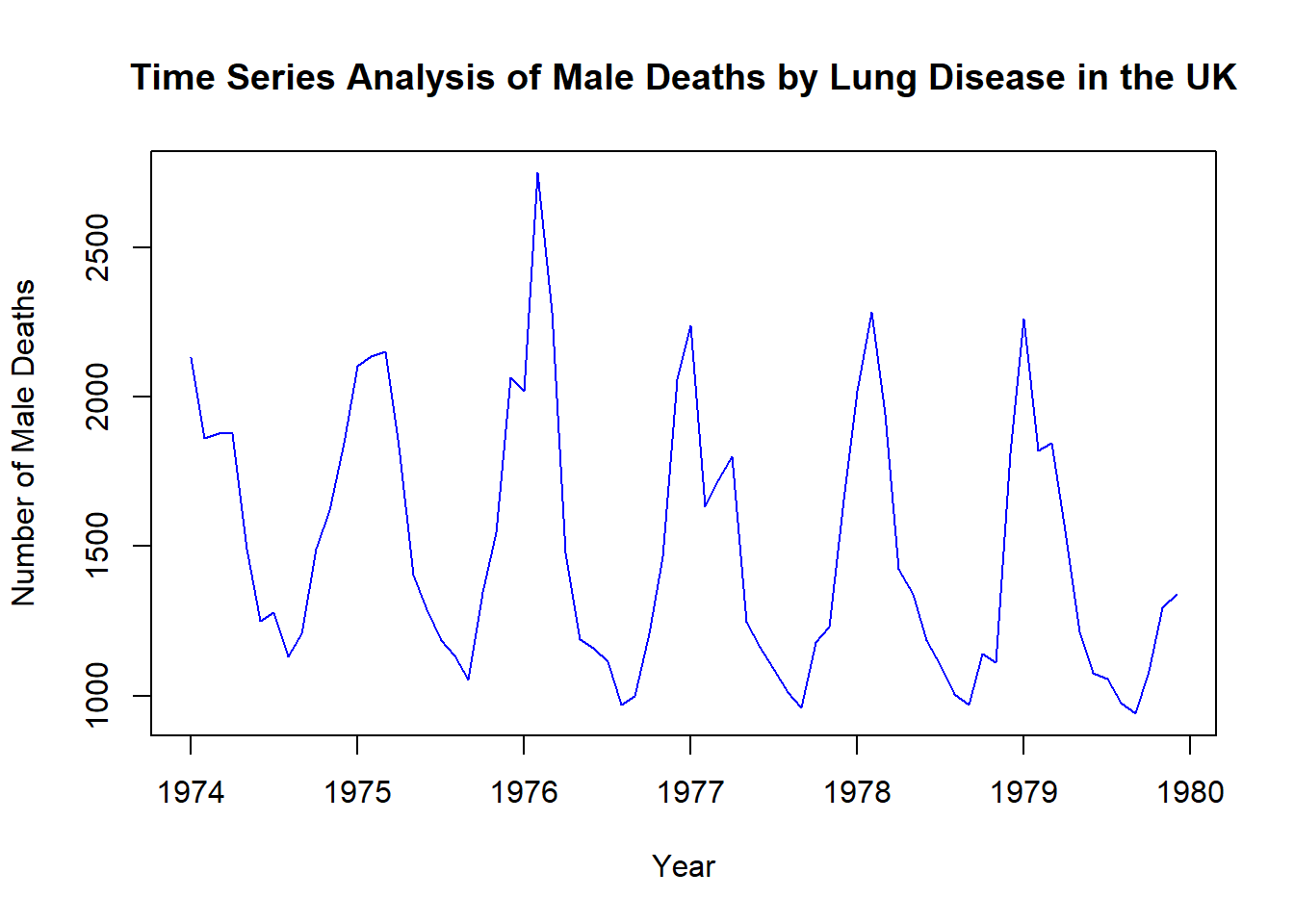
#mdeaths_tsibbleTo recover seasonality separately from the long run trend, I will use a classical decomposition. This will allow me to break total deaths \(D_t\) into a trend component \(T_t\), a seasonal component \(S_t\), and a random component \(R_t\). I will make the assumption that an additive model describes our data, as I don’t see evidence in the above plot that the magnitude of seasonality is changing over time:
\[D_t = S_t + T_t + R_t\] To understand this decomposition, I’ll make a plot which shows the time series in the raw data, the long run trend, the seasonal component, and the remainder random component.
mdeaths_tsibble |>
  model(classical_decomposition(value, type = "additive")) |>
  components() |>
  autoplot() +
  labs(title =  "Time Series Analysis of Male Deaths by Lung Disease in the UK")
Warning: Removed 6 rows containing missing values (`geom_line()`).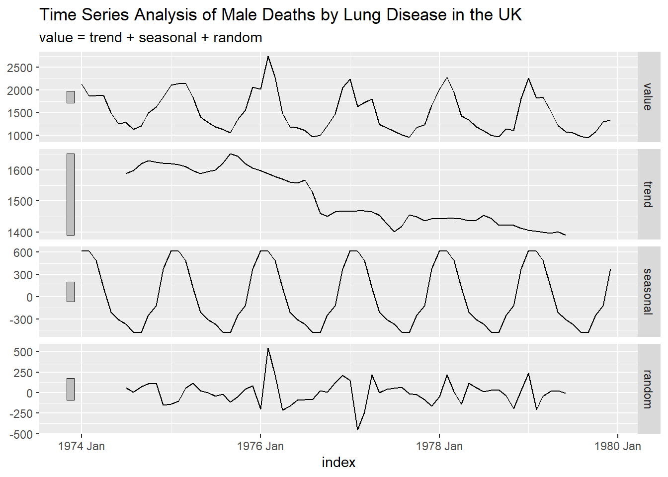
The grey bars on the side of the decomposition plot are there to help assess how “big” each component is. Since the* y*-axes vary across each plot, it’s hard to compare the magnitude of a trend or a seasonal cycle across plots without these grey bars. All grey bars are of the same magnitude; here, about 250. So, when the bar is small relative to the variation shown in a plot, that means that component is quantitatively important in determining overall variation.
There is evidence for a long-run downward trend over time, but it is not greatly contributing to the overall variation in the value. There is evidence of seasonality, exhibited by the cyclical nature of the curve in the seasonality section. The seasonal component is more important in driving overall variation in male lung disease deaths.
@online{favre2022,
  author = {Favre, Kiran},
  title = {Lung {Disease} in the {United} {Kingdom}},
  date = {2022-11-18},
  url = {https://kiranfavre.github.io/posts/2023-11-18_timeseries/},
  langid = {en}
}